
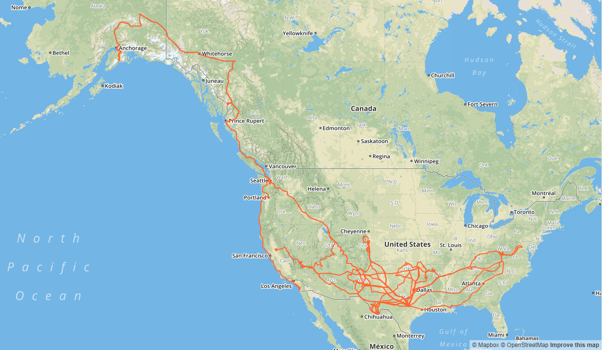
In 2015, as my then-employer was transitioning to fully remote “working from home,” I went on a wild roadtrip with some good friends. It got me thinking: what if that could mean “working from anywhere?” As folks start to see distributed work in their futures, a few friends have asked me how I put these trips together.
I think it’s easier to have a plan that I have no attachment to keeping rather than constantly winging it, so I usually make a rough itinerary. I only find meticulous planning to be important when I’m working on the road.
In those cases, I work days and drive nights. That adds logistical constraints: the drive can’t be too late for “a school night” and stop-overs need to be good places where I’ll be able to get in a solid day’s work in a professional environment — often with friends or family, hotel rooms/lobbies, or coworking spaces. Call quality can significantly drop off in coffee shops and restaurants; libraries or other public spaces can be a gamble. Having a backup plan and a hotspot is useful, too.

And in my unsolicited opinion on the virtues of the digital nomad: don’t fake it. Building good distributed work culture offers the opportunity to re-evaluate what truly makes people productive and collaborative. Let’s avoid giving leaders reasons to backtrack to unhealthy “butts-in-chairs” performance monitoring.
So in celebration of 5 years since the Pacific Coast Highway, I offer up my itinerary template.
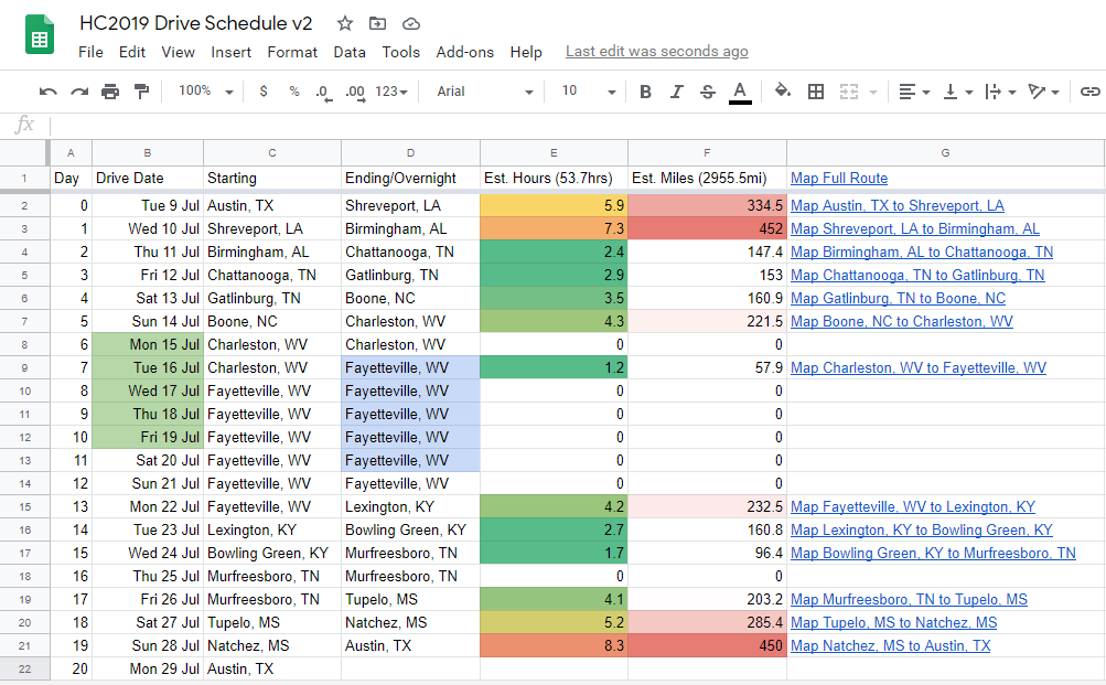
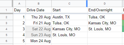
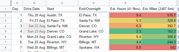
This is a lot less work than it appears — most of it is calculated. I just pick a start date and city, then fill in stops along the way (Column D). The spreadsheet automatically fetches the estimated time and mileage for each row from the Google Maps Directions API. This makes it easy to play with alternate routes or shift hours between days. Last summer, I had to work during a one-way run to Seattle before a vacation, here are the routes I compared:
Those numbers are based on default highway routes. I often prefer something more interesting, but this is great for low-effort feasibility estimates. Besides, the value of a scenic route can drop off pretty hard once it’s dark out. And for being just an estimate, it’s surprisingly accurate.
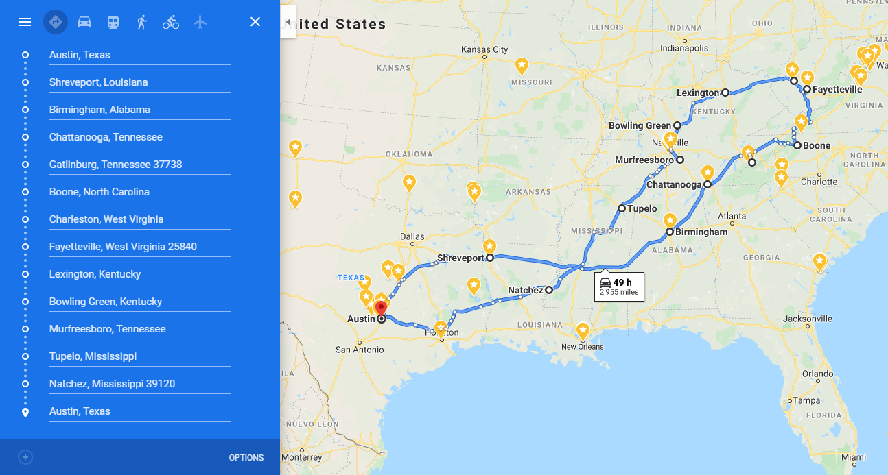
There’s also a link to the full route in the header, but that only works because of a bug in Google Maps — on the website, it is not possible to construct directions for more than 10 stops, but it will accept links to longer itineraries. For now. They will probably fix that.
How to use this
Grab two things: my template and a Google Maps Directions API key.
- Magic Roadtrip Spreadsheet Template v1.3 — Under the “File” menu, select “Make a Copy” to save an editable copy in your Google Drive.
- Google Maps Directions API Key — This requires a developer and billing
account, though the free tier is beyond sufficient for this level of usage.
Google has some good documentation to get started:
- Directions API: “Get an API Key”
- “Get Started with Google Maps Platform” which includes a one-click Get Started.
- (If you know me personally, I’m happy to provision a key for you. I just can’t put it up on the internet unprotected.)
Once you have a key:
- Add your API key in the “Config” tab’s cell
B2 - Go back to the “Route Plan” tab and add:
- Start date in
B2 - Start city in
C2 - Start picking destinations in column
D - To stay more than one night in a city, just repeat that city name in each row.
- Start date in
Be careful not to drag or cut cells in Column D; that will break formulas. Just overwrite or copy-then-paste. Columns A through C (except the first row) and E through G are all auto-calculated. If you try to edit these, there will be a warning. To disable that warning, open “Protected Sheets and Ranges” in the Data menu to remove the block so you can edit freely.
How it works
The magic columns are E and F, and both work using the
IMPORTXML() function
to query Google Maps Directions API and traverse the XML response to find the
answer. To pick apart an example:
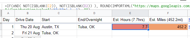
The formula for E2 is:
=IF(
AND( NOT(ISBLANK(C2)), NOT(ISBLANK(D2)), NOT(C2=D2) ),
ROUND(
IMPORTXML(
"https://maps.googleapis.com/maps/api/directions/xml?" &
"origin=" & C2 &
"&destination=" & D2 &
"&key=" & APIKEY & "®ion=us&mode=driving", "//leg/duration/value")
/60/60*1.1, 1
),
"")
First, it checks if there is a drive on this day — are C2 (Austin, TX) and D2
(Tulsa, OK) both filled in and not the same? If so, IMPORTXML runs a
query. The response includes the full directions with a route summary. The
spreadsheet pulls the durationg and distances values from there.
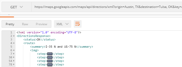
See the xpath_query argument "//leg/duration/value".
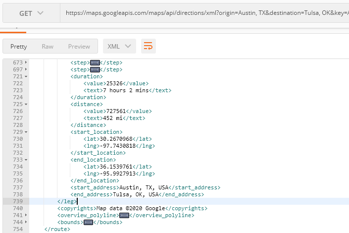
For “Estimated Hours,” it grabs value from the duration (seconds) and —
looking back at the cell formula — converts it to hours and adds 10%
(/60/60*1.1), then rounds it to the nearest tenth with ROUND(value, 1).
=IF(
AND( NOT(ISBLANK(C2)), NOT(ISBLANK(D2)), NOT(C2=D2) ),
ROUND(
IMPORTXML(
"https://maps.googleapis.com/maps/api/directions/xml" &
"?origin=" & C2 &
"&destination="& D2 &
"&key=" & APIKEY &
"®ion=us&mode=driving", "//leg/distance/value")
/1609, 1
),
"")
For “Estimated Miles”, the formula is similar, except IMPORTXML looks for the
value (meters) from distance instead, converts it to miles (/1609),
and rounds it.
In both cases, using the numeric value instead of the text string (“7 hours
2 minutes” or “452 mi”) allows two things: being able to sum them for
totals and apply conditional formatting based on length.
Column G, the map between stops, just does some basic cell references:
=IF(
  AND( NOT(ISBLANK(C2)), NOT(ISBLANK(D2)), NOT(C2 = D2) ),
  HYPERLINK(
    "https://www.google.com/maps/dir/" & C2 & "/" & D2 & "/",
    "Map " & C2 & " to " & D2)
  , "")
The HYPERLINK()
function does “make a link to directions from Cx to Dx and label it ‘Map Cx to
Dx’.”
Columns A, B, and C? Simpler calculations. A and B both “add one to the row
above” — Google Sheets is smart enough to properly handle [date] + 1
correctly. C copies diagonally from the previous row’s Column D.
Named Ranges and Conditional Formatting
The second tab in the spreadsheet is a worksheet called “Config.” This is where you add your API key and preferences about drive times. All of these are defined as Named Ranges so that they can be used in formulas easily:
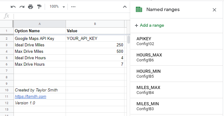
This is how the formulas in the last section were able to reference APIKEY
instead of writing the key directly into the cell formula or doing a
cross-sheet reference like Config!B2. These named ranges are also used in
conditional formatting, but there’s a trick to that.
Conditional Formatting is applied to columns B, E, and F. Column B highlights weekends. Columns E and F use the named ranges from “Config” to apply color to ideal/max driving distance/time.
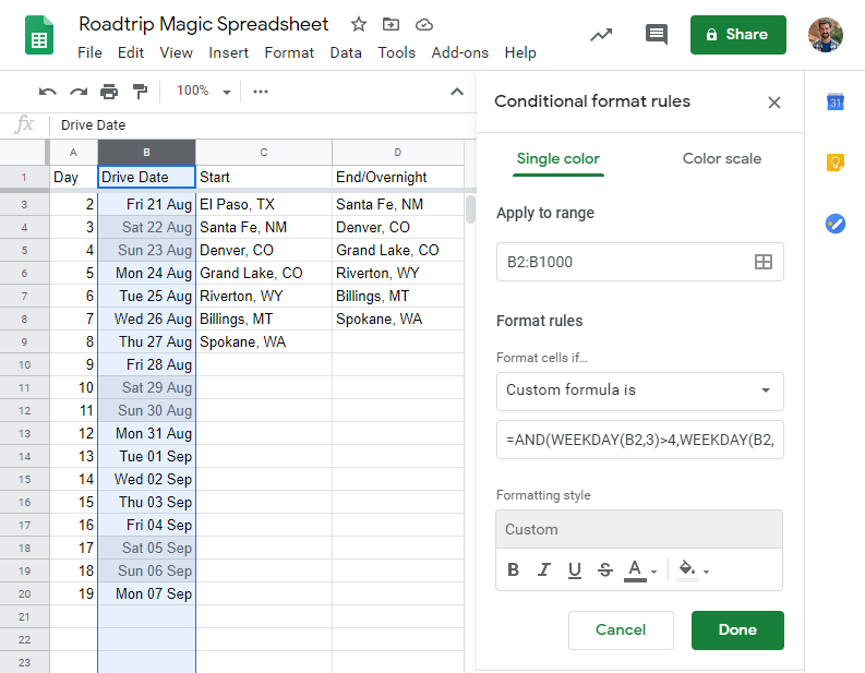
Conditional formatting to highlight weekends uses
WEEKDAY() to format
B2:B with this custom formula:
=AND(WEEKDAY(B2,3)>4,WEEKDAY(B2,3)<7)
The WEEKDAY() function gets numbers for day-of-the-week. It has different
modes: in mode 3, Saturday translates to 5 and Sunday is 6.
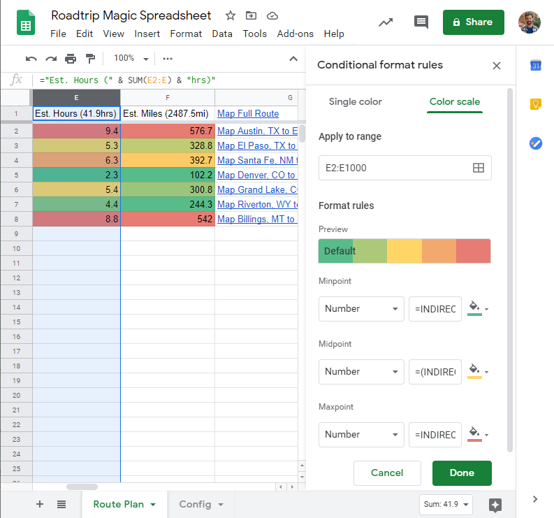
For E and F, the conditional formatting compares against the named ranges in the
Config tab. Neither cross-sheet references (i.e. Sheet!A1) nor named ranges
can be used in formatting formulas directly. Instead, they have to be referenced
through INDIRECT().
Minpoint:
=INDIRECT("HOURS_MIN")

Midpoint:
=(INDIRECT("HOURS_MIN")+INDIRECT("HOURS_MAX"))/2

Maxpoint:
=INDIRECT("HOURS_MAX")
Take it for a spin
Grab a copy, take it for a test drive, and let me know what you think. Plan something crazy. Go somewhere you’ve never heard of. Work from a cabin in the woods for a while. See you out there!
Magic Roadtrip Spreadsheet Template v1.3
In this time, I do feel compelled to add: I’ve had this post in the hopper for a while. Circumstances have since changed. Please consider the impact any travel has on community spread and the disproportionate effects on remote communities. I know I’m certainly looking forward to travel re-unleashed one day. Until then, we must step lightly and acknowledge how leave-no-trace has taken on a whole new meaning.

Template Changelog
- v1.3
- Add red highlighting and an error message in the header row if the API key is missing. Add link to blog post for instructions in Config sheet.
- v1.2
- Add the “stopover detection” from Column G into E and F, preventing API calls on rows with the same start and stop points.
- Update Conditional Formatting so that 0 miles/hours days are greyed out instead of green.
- v1.0
- Finally consolidate all those copies-of-copies into a template and fix all the broken stuff.